Dragon Dance

What is that?

Dragon Dance is a plugin for Ghidra to get visualize and manipulate the binary code coverage data. Coverage data can be imported from the multiple coverage sources. For now the plugin supports Dynamorio and Intel Pin binary instrumentation tools. Dynamorio has its own coverage collection module called "drcov". Intel Pin does not provide a builtin coverage collector module. To handle the lack of module situation I have to write my own coverage collection module for Intel Pin. So I wrote a coverage collection module for Intel Pin named ddph (Dragon Dance Pin Helper). So you can use that. You can view ddph's source from this link. If you are lazy to compile for your own, you can use the compiled binaries I provided for Windows, macOS and Linux.

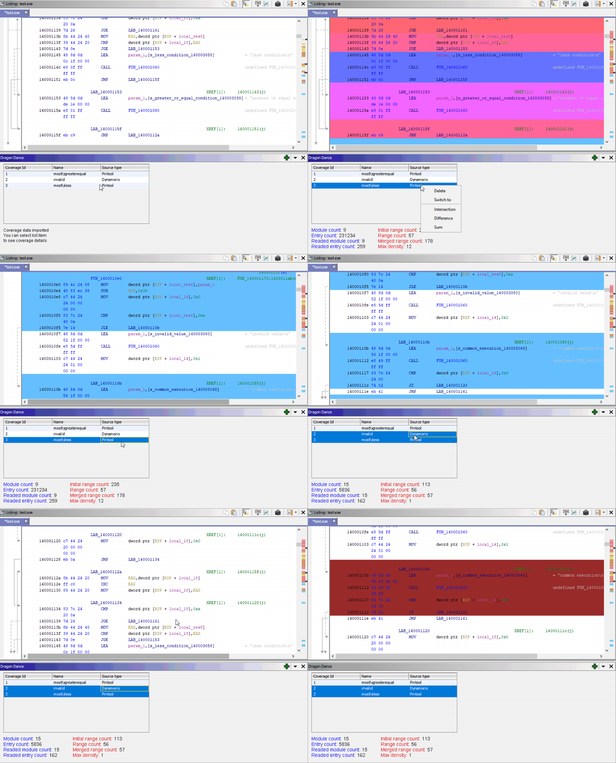
Dragon Dance can import and use multiple coverage data in the same session. (Also it supports multi-session but for now that's not usable by the GUI). And you can switch between them or apply intersection, difference, distinct or sum operation with each other quickly.

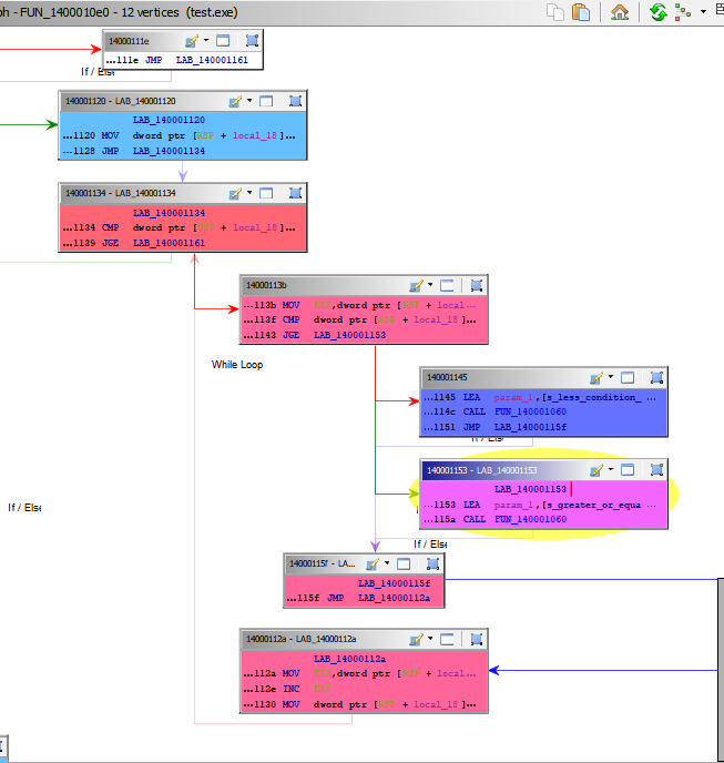
Dragon Dance lets you to view intensity of the executed instructions. So you can get hint on which instructions how often executed. Also you can view the coverage visualization on the function graph window.

Scripting

Dragon Dance also supports its own scripting system.

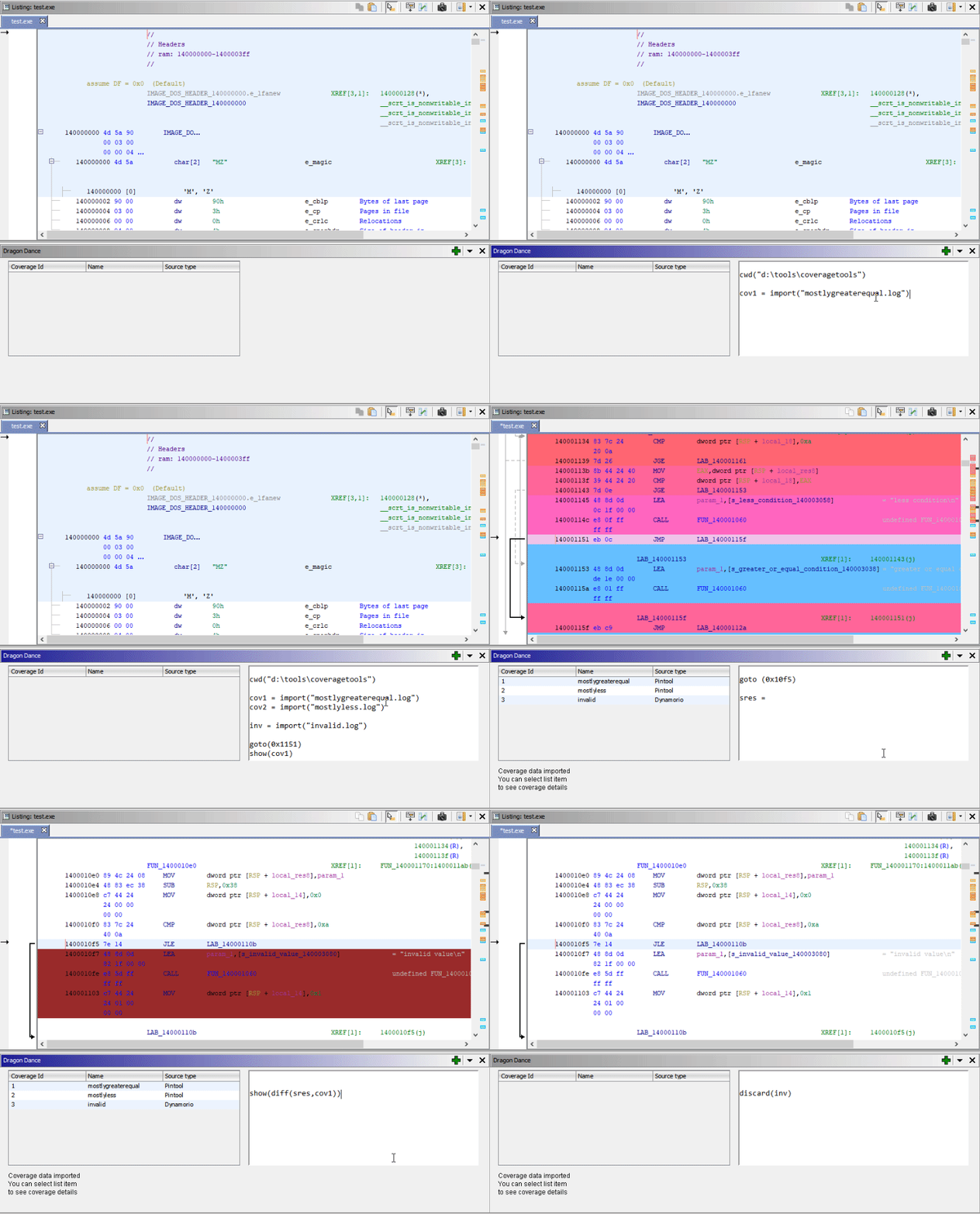
It lets you flexible way to play with the coverage data. You can load, delete, show, intersect, diff, distinct, sum operation on them. Following section will be contained the scripting system and api. Press Alt + Enter keys to execute the script.

Built-in Functions

Built-in functions are implementation of the internal coverage operations to supply an interface to the scripting system. Built-in function can be return coverage object variable or nothing. Built-ins may have aliases.

They are accepts Built-in Arg as a parameter. Parameters can be variable length.

Built-in Arg

Built-in Arg is a reference to hold different type of the value. Built-in Args passed left to right order. Built-in Arg can hold following value types:

• Coverage Data Object (which is returned by Built-ins)
• String
• Integer (Can be decimal, hexadecimal or octal forms)

Variables

Variables are responsible to hold the coverage object only. They can be loaded by built-in functions. They can be passed as an parameter (Built-in Arg) to the Built-in Functions.

There is two types of the coverage object.

Physical Coverage Object and Logical Coverage Object

Physical Coverage Object points a coverage object that it loaded directly from the coverage file. They are visible on the coverage table which is on the GUI. So you can interact them via the GUI operations.

Logical Coverage Object points a coverage object that has processed in a built-in function and returned from it as a result. They are not visible on the GUI but they can lives in a Variable until they are destroyed.

Coverage object maintained by the Variable object automatically for both of type of the coverage object. For example;

cov1 = load("firstcoverage.out")
cov2 = load("secondcov.out")

cov1 = diff(cov1,cov2)

In this example cov1 and cov2 are variable. And both variables has physical coverage object. diff built-in takes both variables and sets the return value to the cov1 variable. That overwrite operation will set the result coverage object to the variable but does not delete the coverage object because that is a physical coverage object. That coverage data will remain in the session and also GUI table.

Let's think previous example like this;

cov1 = load("first.out")
cov2 = load("second.out")
cov3 = load("third.out")
rvar = sum(cov1,cov2,cov3)
rvar = diff(rvar, cov2)

In this example three physical coverage variable goes into sum operation and the sum operation returns logical result coverage object. Then the diff operation takes a logical and a physical variable in it and overwrites the variable named rvar.

In this case, the result will be set to the rvar and it's previous coverage value destroyed immediately. Because this was a logical object and should be deleted to prevent object leakage. If you want to destroy a variable that it contained a physical coverage object, you have to call discard built-in to do. All built-ins will be detailed below.

You can write complex scripts using nested built-in calls, you can write something like so:

cres = diff(intersect(a, load("another.log"), c, d), sum(e,f) )

you don't have to write the logic line by line.

Built-in References

The following API documentations and their behaviors may change until reached final version.

clear()

Property	Description
Return Value	None
Minimum Parameter Count	0
Maximum Parameter Count	0
Description	This built-in clears the being visualized coverage and sets the active coverage to null.
Aliases	None

cwd( String : workingDirectory )

Property	Description
Return Value	None
Minimum Parameter Count	1
Maximum Parameter Count	1
Description	Sets the current working directory with the given path. All import calls without absolute path after the cwd the coverage files will be searched in the active working directory.
Aliases	None

diff( Variable : var1, var2, ..... varN )

Property	Description
Return Value	Variable
Minimum Parameter Count	2
Maximum Parameter Count	Unlimited
Description	Applies difference operation to given variable length Variables. And returns the result coverage variable.
Aliases	None

discard( Variable : var1, var2, ..... varN )